


Alright, let’s talk about my little adventure with Massey ratings. I’d been seeing these kinds of rankings pop up, especially for sports, and got curious about how they actually worked under the hood. Decided the best way to figure it out was just to try and build it myself.
Getting Started: Understanding the Core Idea
So, the first thing I did was dig around to get the basic concept. It wasn’t super complicated at its heart. You basically look at all the games played. For each game, you know who played who and what the score difference was. The whole idea is to use this info to build a big math problem – a system of linear equations, they call it. The solution to this problem gives you the rating for each team.
It made sense: teams that beat others by a lot should have higher ratings, and teams that lose consistently should have lower ones. The math just formalizes this.
Gathering the Raw Material: Game Data
Next up, I needed data. Couldn’t rate teams without knowing how they played. I decided to keep it simple for the first run. I just grabbed some results from a recent season of a sport I follow. Didn’t need anything fancy. I put it into a basic text file, something like:
- Team A, Team B, Score A, Score B
- Team C, Team D, Score C, Score D
- Team A, Team C, Score A, Score C
Just a list of matchups and scores. That was enough to get started.
Building the Math Problem: The Matrix
This was the core part. I had to translate those game results into the Massey matrix (let’s call it M) and a points differential vector (let’s call it p). Here’s how I went about it:
First, I figured out how many teams I had. Let’s say it was ‘n’ teams. I knew I needed an ‘n’ by ‘n’ matrix M, and a vector p with ‘n’ entries. I started with both filled with zeros.
Then, I went through my game list, one game at a time.

- For a game between Team X and Team Y:
- I added 1 to the diagonal spot for Team X (M[X][X]) and Team Y (M[Y][Y]). This basically counts the games played for each team.
- I subtracted 1 from the off-diagonal spots M[X][Y] and M[Y][X]. This links the two teams in the matrix.
- For the vector p, I calculated the point difference. If Team X scored ScoreX and Team Y scored ScoreY, I added (ScoreX – ScoreY) to p[X] and the opposite, (ScoreY – ScoreX), to p[Y].
I repeated this for every single game in my data file. After processing all games, I had my matrix M and vector p populated based on the season’s results.
The Little Hiccup: Fixing the Matrix
Now, I remembered reading that the way this matrix is built makes it impossible to solve directly. Something about it being ‘rank deficient’. The common fix seemed pretty straightforward, though. I just took the very last row of my matrix M and replaced all its entries with 1. Then, I set the very last entry in my vector p to 0. This apparently anchors the ratings and makes the system solvable. Felt a bit like a hack, but hey, if it works, it works.
Finding the Answer: Solving for Ratings
With the matrix M and vector p ready and adjusted, the final step was to solve the equation M r = p for ‘r’. This ‘r’ vector would hold the actual Massey ratings for each team.
I’m not gonna lie, I didn’t do this by hand. I used a programming language, Python, and its numerical library called NumPy. It has built-in functions to solve these kinds of linear systems. I fed it my matrix M and vector p, and it spat out the ratings vector r.
Looking at the Results
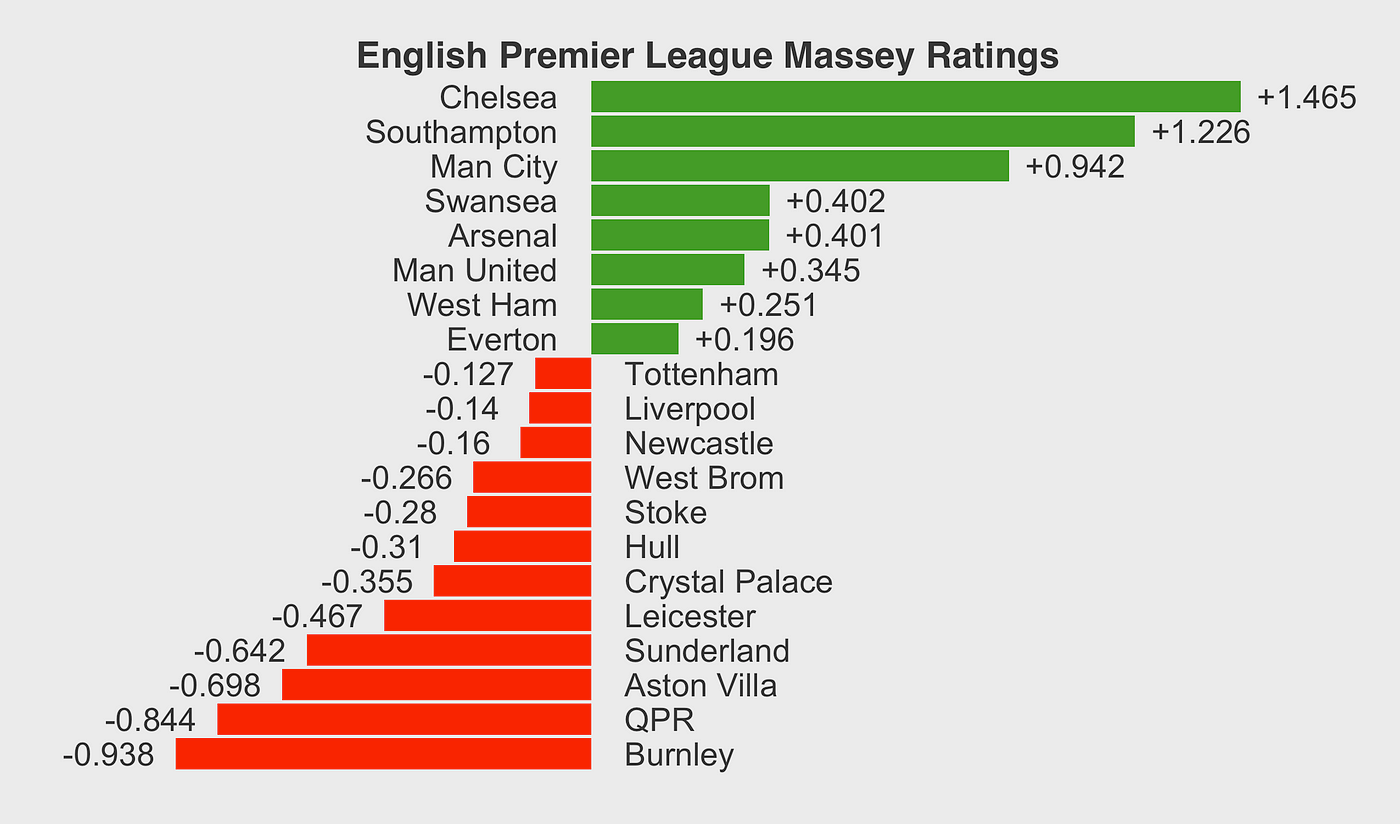
And there it was! A list of numbers, one for each team. Higher numbers meant better ratings according to the Massey system. I spent some time looking at the rankings it produced. Did they make sense? Mostly, yeah. Teams with strong records and big wins were near the top, and teams that struggled were near the bottom. It felt pretty good to see the raw data turned into a meaningful ranking through this process.

It wasn’t perfect, maybe some rankings seemed a bit off here or there, but it was a solid first attempt. Implementing it myself definitely made me understand how it works way better than just reading about it.


